Loading and working with GeoMIP (G6sulfur) data directly from ESGF#
This notebook demonstrates how to load and analyze GeoMIP (Geoengineering Model Intercomparison Project) G6sulfur data directly from ESGF, comparing it with standard climate scenarios.
Install required packages (
intake_esgf,xmip)Search for G6sulfur and comparison scenarios (SSP2-4.5, SSP5-8.5)
Load data and apply preprocessing with
xmipCalculate global means and annual resampling
Visualize temperature trajectories under different scenarios
Install required packages#
We need two key packages:
intake_esgf: For searching and loading data from ESGF nodesxmip: For preprocessing CMIP6 data (renaming variables, handling coordinates, etc.)
The xmip package is particularly useful for standardizing CMIP6 data across different models and experiments.
# on starting the server, we need to run the line below once, as intake_esgf is not yet in our standard pangeo environment
# but it can be commented out after this, to save time
%pip install intake_esgf
%pip install xmip
Requirement already satisfied: intake_esgf in /Users/susannebaur/miniconda3/envs/CloudHub/lib/python3.13/site-packages (2025.9.26)
Requirement already satisfied: dask>=2024.12.0 in /Users/susannebaur/miniconda3/envs/CloudHub/lib/python3.13/site-packages (from intake_esgf) (2025.9.1)
Requirement already satisfied: globus-sdk>=3.49.0 in /Users/susannebaur/miniconda3/envs/CloudHub/lib/python3.13/site-packages (from intake_esgf) (3.64.0)
Requirement already satisfied: netcdf4>=1.7.2 in /Users/susannebaur/miniconda3/envs/CloudHub/lib/python3.13/site-packages (from intake_esgf) (1.7.2)
Requirement already satisfied: pandas>=2.2.3 in /Users/susannebaur/miniconda3/envs/CloudHub/lib/python3.13/site-packages (from intake_esgf) (2.3.2)
Requirement already satisfied: pystac-client>=0.8.6 in /Users/susannebaur/miniconda3/envs/CloudHub/lib/python3.13/site-packages (from intake_esgf) (0.9.0)
Requirement already satisfied: pyyaml>=6.0.2 in /Users/susannebaur/miniconda3/envs/CloudHub/lib/python3.13/site-packages (from intake_esgf) (6.0.2)
Requirement already satisfied: requests>=2.32.3 in /Users/susannebaur/miniconda3/envs/CloudHub/lib/python3.13/site-packages (from intake_esgf) (2.32.4)
Requirement already satisfied: requests-cache>=1.2.1 in /Users/susannebaur/miniconda3/envs/CloudHub/lib/python3.13/site-packages (from intake_esgf) (1.2.1)
Requirement already satisfied: tqdm>=4.67.1 in /Users/susannebaur/miniconda3/envs/CloudHub/lib/python3.13/site-packages (from intake_esgf) (4.67.1)
Requirement already satisfied: xarray>=2024.11.0 in /Users/susannebaur/miniconda3/envs/CloudHub/lib/python3.13/site-packages (from intake_esgf) (2025.4.0)
Requirement already satisfied: click>=8.1 in /Users/susannebaur/miniconda3/envs/CloudHub/lib/python3.13/site-packages (from dask>=2024.12.0->intake_esgf) (8.2.1)
Requirement already satisfied: cloudpickle>=3.0.0 in /Users/susannebaur/miniconda3/envs/CloudHub/lib/python3.13/site-packages (from dask>=2024.12.0->intake_esgf) (3.1.1)
Requirement already satisfied: fsspec>=2021.09.0 in /Users/susannebaur/miniconda3/envs/CloudHub/lib/python3.13/site-packages (from dask>=2024.12.0->intake_esgf) (2025.7.0)
Requirement already satisfied: packaging>=20.0 in /Users/susannebaur/miniconda3/envs/CloudHub/lib/python3.13/site-packages (from dask>=2024.12.0->intake_esgf) (25.0)
Requirement already satisfied: partd>=1.4.0 in /Users/susannebaur/miniconda3/envs/CloudHub/lib/python3.13/site-packages (from dask>=2024.12.0->intake_esgf) (1.4.2)
Requirement already satisfied: toolz>=0.10.0 in /Users/susannebaur/miniconda3/envs/CloudHub/lib/python3.13/site-packages (from dask>=2024.12.0->intake_esgf) (1.0.0)
Requirement already satisfied: pyjwt<3.0.0,>=2.0.0 in /Users/susannebaur/miniconda3/envs/CloudHub/lib/python3.13/site-packages (from pyjwt[crypto]<3.0.0,>=2.0.0->globus-sdk>=3.49.0->intake_esgf) (2.10.1)
Requirement already satisfied: cryptography!=3.4.0,>=3.3.1 in /Users/susannebaur/miniconda3/envs/CloudHub/lib/python3.13/site-packages (from globus-sdk>=3.49.0->intake_esgf) (46.0.1)
Requirement already satisfied: charset_normalizer<4,>=2 in /Users/susannebaur/miniconda3/envs/CloudHub/lib/python3.13/site-packages (from requests>=2.32.3->intake_esgf) (3.4.3)
Requirement already satisfied: idna<4,>=2.5 in /Users/susannebaur/miniconda3/envs/CloudHub/lib/python3.13/site-packages (from requests>=2.32.3->intake_esgf) (3.10)
Requirement already satisfied: urllib3<3,>=1.21.1 in /Users/susannebaur/miniconda3/envs/CloudHub/lib/python3.13/site-packages (from requests>=2.32.3->intake_esgf) (2.5.0)
Requirement already satisfied: certifi>=2017.4.17 in /Users/susannebaur/miniconda3/envs/CloudHub/lib/python3.13/site-packages (from requests>=2.32.3->intake_esgf) (2025.8.3)
Requirement already satisfied: cffi>=2.0.0 in /Users/susannebaur/miniconda3/envs/CloudHub/lib/python3.13/site-packages (from cryptography!=3.4.0,>=3.3.1->globus-sdk>=3.49.0->intake_esgf) (2.0.0)
Requirement already satisfied: pycparser in /Users/susannebaur/miniconda3/envs/CloudHub/lib/python3.13/site-packages (from cffi>=2.0.0->cryptography!=3.4.0,>=3.3.1->globus-sdk>=3.49.0->intake_esgf) (2.23)
Requirement already satisfied: cftime in /Users/susannebaur/miniconda3/envs/CloudHub/lib/python3.13/site-packages (from netcdf4>=1.7.2->intake_esgf) (1.6.4.post1)
Requirement already satisfied: numpy in /Users/susannebaur/miniconda3/envs/CloudHub/lib/python3.13/site-packages (from netcdf4>=1.7.2->intake_esgf) (2.3.2)
Requirement already satisfied: python-dateutil>=2.8.2 in /Users/susannebaur/miniconda3/envs/CloudHub/lib/python3.13/site-packages (from pandas>=2.2.3->intake_esgf) (2.9.0.post0)
Requirement already satisfied: pytz>=2020.1 in /Users/susannebaur/miniconda3/envs/CloudHub/lib/python3.13/site-packages (from pandas>=2.2.3->intake_esgf) (2025.2)
Requirement already satisfied: tzdata>=2022.7 in /Users/susannebaur/miniconda3/envs/CloudHub/lib/python3.13/site-packages (from pandas>=2.2.3->intake_esgf) (2025.2)
Requirement already satisfied: locket in /Users/susannebaur/miniconda3/envs/CloudHub/lib/python3.13/site-packages (from partd>=1.4.0->dask>=2024.12.0->intake_esgf) (1.0.0)
Requirement already satisfied: pystac>=1.10.0 in /Users/susannebaur/miniconda3/envs/CloudHub/lib/python3.13/site-packages (from pystac[validation]>=1.10.0->pystac-client>=0.8.6->intake_esgf) (1.14.1)
Requirement already satisfied: jsonschema~=4.18 in /Users/susannebaur/miniconda3/envs/CloudHub/lib/python3.13/site-packages (from pystac[validation]>=1.10.0->pystac-client>=0.8.6->intake_esgf) (4.25.0)
Requirement already satisfied: attrs>=22.2.0 in /Users/susannebaur/miniconda3/envs/CloudHub/lib/python3.13/site-packages (from jsonschema~=4.18->pystac[validation]>=1.10.0->pystac-client>=0.8.6->intake_esgf) (25.3.0)
Requirement already satisfied: jsonschema-specifications>=2023.03.6 in /Users/susannebaur/miniconda3/envs/CloudHub/lib/python3.13/site-packages (from jsonschema~=4.18->pystac[validation]>=1.10.0->pystac-client>=0.8.6->intake_esgf) (2025.4.1)
Requirement already satisfied: referencing>=0.28.4 in /Users/susannebaur/miniconda3/envs/CloudHub/lib/python3.13/site-packages (from jsonschema~=4.18->pystac[validation]>=1.10.0->pystac-client>=0.8.6->intake_esgf) (0.36.2)
Requirement already satisfied: rpds-py>=0.7.1 in /Users/susannebaur/miniconda3/envs/CloudHub/lib/python3.13/site-packages (from jsonschema~=4.18->pystac[validation]>=1.10.0->pystac-client>=0.8.6->intake_esgf) (0.27.0)
Requirement already satisfied: six>=1.5 in /Users/susannebaur/miniconda3/envs/CloudHub/lib/python3.13/site-packages (from python-dateutil>=2.8.2->pandas>=2.2.3->intake_esgf) (1.17.0)
Requirement already satisfied: cattrs>=22.2 in /Users/susannebaur/miniconda3/envs/CloudHub/lib/python3.13/site-packages (from requests-cache>=1.2.1->intake_esgf) (25.2.0)
Requirement already satisfied: platformdirs>=2.5 in /Users/susannebaur/miniconda3/envs/CloudHub/lib/python3.13/site-packages (from requests-cache>=1.2.1->intake_esgf) (4.3.8)
Requirement already satisfied: url-normalize>=1.4 in /Users/susannebaur/miniconda3/envs/CloudHub/lib/python3.13/site-packages (from requests-cache>=1.2.1->intake_esgf) (2.2.1)
Requirement already satisfied: typing-extensions>=4.12.2 in /Users/susannebaur/miniconda3/envs/CloudHub/lib/python3.13/site-packages (from cattrs>=22.2->requests-cache>=1.2.1->intake_esgf) (4.14.1)
Note: you may need to restart the kernel to use updated packages.
We look at global mean temperature trajectories for three scenarios:
SSP2-4.5: Moderate emissions scenario (baseline)
SSP5-8.5: High emissions scenario (worst case)
G6sulfur: Geoengineering scenario (aerosol injection)
import os
import glob
import pandas as pd
import numpy as np
import xarray as xr
from xmip.preprocessing import rename_cmip6
import matplotlib
import matplotlib.pyplot as plt
from tqdm import tqdm
import intake_esgf
#from utils import weighted_seasonal_resample, weighted_annual_resample, calc_weighted_spatial_means
import warnings
warnings.filterwarnings("ignore", module='xarray') # not great practice, but xarray tends to give lots of verbose warnings

# user inputs
scenarios = ['ssp245', 'ssp585', 'G6sulfur']


# time-periods over which to take means
assessment_periods = {'Future':slice('2080', '2099'),
                      'Baseline':slice('2015', '2034')}
intake_esgf.conf.set(all_indices=True)
cat = intake_esgf.ESGFCatalog()
cat.search(
    project='CMIP6',
    experiment_id=scenarios,
    source_id='UKESM1-0-LL',
    variable_id='tas',  # surface air temperature
    table_id='Amon',    # monthly atmospheric data
    variant_label=['r1i1p1f2']  # ensemble member
)
Summary information for 3 results:
mip_era                              [CMIP6]
activity_drs           [ScenarioMIP, GeoMIP]
institution_id                        [MOHC]
source_id                      [UKESM1-0-LL]
experiment_id     [ssp245, ssp585, G6sulfur]
member_id                         [r1i1p1f2]
table_id                              [Amon]
variable_id                            [tas]
grid_label                              [gn]
dtype: object
Load data with preprocessing#
The to_dataset_dict(add_measures=True) method:
Downloads data from ESGF nodes
Applies
xmippreprocessing to standardize variable names and coordinatesCreates a dictionary with keys for each experiment (e.g., ‘ScenarioMIP.ssp245’, ‘GeoMIP.G6sulfur’)
The add_measures=True parameter ensures we get additional metadata and measures for proper analysis.
dsd = cat.to_dataset_dict(add_measures=True)
Downloading 132.4 [Mb]...
{'ScenarioMIP.ssp245': <xarray.Dataset> Size: 120MB
 Dimensions:    (time: 1032, bnds: 2, lat: 144, lon: 192)
 Coordinates:
   * time       (time) object 8kB 2015-01-16 00:00:00 ... 2100-12-16 00:00:00
   * lat        (lat) float64 1kB -89.38 -88.12 -86.88 ... 86.88 88.12 89.38
   * lon        (lon) float64 2kB 0.9375 2.812 4.688 6.562 ... 355.3 357.2 359.1
     height     float64 8B 1.5
 Dimensions without coordinates: bnds
 Data variables:
     time_bnds  (time, bnds) object 17kB dask.array<chunksize=(1, 2), meta=np.ndarray>
     lat_bnds   (time, lat, bnds) float64 2MB dask.array<chunksize=(420, 144, 2), meta=np.ndarray>
     lon_bnds   (time, lon, bnds) float64 3MB dask.array<chunksize=(420, 192, 2), meta=np.ndarray>
     tas        (time, lat, lon) float32 114MB dask.array<chunksize=(1, 144, 192), meta=np.ndarray>
     areacella  (lat, lon) float32 111kB ...
 Attributes: (12/48)
     Conventions:            CF-1.7 CMIP-6.2
     activity_id:            ScenarioMIP
     branch_method:          standard
     branch_time_in_child:   59400.0
     branch_time_in_parent:  59400.0
     creation_date:          2019-04-18T14:21:20Z
     ...                     ...
     variant_label:          r1i1p1f2
     license:                CMIP6 model data produced by the Met Office Hadle...
     cmor_version:           3.4.0
     tracking_id:            hdl:21.14100/53ca95cf-f8c8-4606-9d5b-2ba5e10907f0
     activity_drs:           ScenarioMIP
     member_id:              r1i1p1f2,
 'ScenarioMIP.ssp585': <xarray.Dataset> Size: 120MB
 Dimensions:    (time: 1032, bnds: 2, lat: 144, lon: 192)
 Coordinates:
   * time       (time) object 8kB 2015-01-16 00:00:00 ... 2100-12-16 00:00:00
   * lat        (lat) float64 1kB -89.38 -88.12 -86.88 ... 86.88 88.12 89.38
   * lon        (lon) float64 2kB 0.9375 2.812 4.688 6.562 ... 355.3 357.2 359.1
     height     float64 8B 1.5
 Dimensions without coordinates: bnds
 Data variables:
     time_bnds  (time, bnds) object 17kB dask.array<chunksize=(1, 2), meta=np.ndarray>
     lat_bnds   (time, lat, bnds) float64 2MB dask.array<chunksize=(420, 144, 2), meta=np.ndarray>
     lon_bnds   (time, lon, bnds) float64 3MB dask.array<chunksize=(420, 192, 2), meta=np.ndarray>
     tas        (time, lat, lon) float32 114MB dask.array<chunksize=(1, 144, 192), meta=np.ndarray>
     areacella  (lat, lon) float32 111kB ...
 Attributes: (12/48)
     Conventions:            CF-1.7 CMIP-6.2
     activity_id:            ScenarioMIP
     branch_method:          standard
     branch_time_in_child:   59400.0
     branch_time_in_parent:  59400.0
     creation_date:          2019-04-18T14:32:46Z
     ...                     ...
     variant_label:          r1i1p1f2
     license:                CMIP6 model data produced by the Met Office Hadle...
     cmor_version:           3.4.0
     tracking_id:            hdl:21.14100/99449bbe-e9f9-4da7-aff6-b0e95a6e51ac
     activity_drs:           ScenarioMIP
     member_id:              r1i1p1f2,
 'GeoMIP.G6sulfur': <xarray.Dataset> Size: 113MB
 Dimensions:    (time: 972, bnds: 2, lat: 144, lon: 192)
 Coordinates:
   * time       (time) object 8kB 2020-01-16 00:00:00 ... 2100-12-16 00:00:00
   * lat        (lat) float64 1kB -89.38 -88.12 -86.88 ... 86.88 88.12 89.38
   * lon        (lon) float64 2kB 0.9375 2.812 4.688 6.562 ... 355.3 357.2 359.1
     height     float64 8B 1.5
 Dimensions without coordinates: bnds
 Data variables:
     time_bnds  (time, bnds) object 16kB dask.array<chunksize=(1, 2), meta=np.ndarray>
     lat_bnds   (time, lat, bnds) float64 2MB dask.array<chunksize=(360, 144, 2), meta=np.ndarray>
     lon_bnds   (time, lon, bnds) float64 3MB dask.array<chunksize=(360, 192, 2), meta=np.ndarray>
     tas        (time, lat, lon) float32 107MB dask.array<chunksize=(1, 144, 192), meta=np.ndarray>
     areacella  (lat, lon) float32 111kB ...
 Attributes: (12/49)
     Conventions:            CF-1.7 CMIP-6.2
     activity_id:            GeoMIP
     branch_method:          standard
     branch_time_in_child:   61200.0
     branch_time_in_parent:  61200.0
     creation_date:          2019-11-12T11:49:10Z
     ...                     ...
     variant_label:          r1i1p1f2
     license:                CMIP6 model data produced by the Met Office Hadle...
     cmor_version:           3.4.0
     tracking_id:            hdl:21.14100/a2ed4698-3b65-44d8-8599-99490b5b6155
     activity_drs:           GeoMIP
     member_id:              r1i1p1f2}
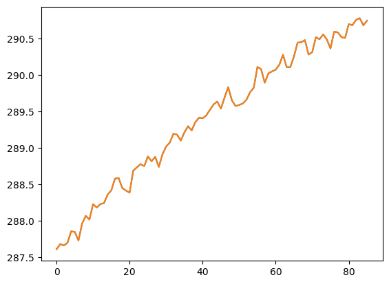
plt.plot(global_mean(dsd['ScenarioMIP.ssp245'], 'tas').resample(time='AS').mean().tas)
[<matplotlib.lines.Line2D at 0x7f2bb821da60>]
Example Usage#
We define two key functions for our analysis:
global_mean(): Calculates area-weighted global means using the areacella variable (grid cell areas) to account for the varying size of grid cells at different latitudes.
weighted_annual_resample(): Converts monthly data to annual means using day-of-month weights to account for different month lengths (e.g., February vs. March).
## example usage, lets plot the global spatial mean timeseries under the three scenarios:

# first, define a function to get the global mean, accounting for area weights (areacella)
def global_mean(ds, variable):
    weights = ds['areacella']
    data = ds[variable]

    # Normalize weights to sum to 1
    weights_normalized = weights / weights.sum()

    # Apply weighted mean
    global_mean = (data * weights_normalized).sum(dim=['lat', 'lon'])

    return global_mean.to_dataset(name=variable)

# second, define a function to resample to annual resolution
# note, in general we have to account for different month lengths
def weighted_annual_resample(ds):
    """
    weight by days in each month
    adapted from NCAR docs
    https://ncar.github.io/esds/posts/2021/yearly-averages-xarray/
    """
    # Determine the month length
    month_length = ds.time.dt.days_in_month

    # Calculate the weights
    wgts = month_length.groupby("time.year") / month_length.groupby("time.year").sum()

    # Make sure the weights in each year add up to 1
    np.testing.assert_allclose(wgts.groupby("time.year").sum(xr.ALL_DIMS), 1.0)

    numerator = (ds * wgts).resample(time="YS").sum(dim="time")
    denominator = wgts.resample(time="YS").sum(dim="time")

    return numerator/denominator
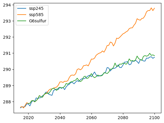
Compare temperature trajectories#
# make a quick plot:

for scenario in ['ScenarioMIP.ssp245', 'ScenarioMIP.ssp585', 'GeoMIP.G6sulfur']:
    data = weighted_annual_resample(global_mean(dsd[scenario], 'tas'))
    plt.plot(data.time.dt.year, data.tas, label=scenario.split('.')[1])
plt.legend()
<matplotlib.legend.Legend at 0x7f2b97965d90>
Resources: