
ARISE 3-D multi-variable analysis — SSP245-TSMLT-GAUSS-DEFAULT#
Analyses multiple 3-D monthly variables from the CESM2-WACCM SSP245-TSMLT-GAUSS-DEFAULT scenario hosted on the NCAR ARISE AWS S3 bucket.
Data source:
Variables processed: can be anything, here starting with so4_a1, so4_a2, so4_a3, dgnumwet1, dgnumwet2, dgnumwet3, REFF_AERO, OH
Memory strategy: files are opened lazily with dask (chunks={'time': 12}) so the full 8 GB is never loaded into RAM. Only the reduced quantities (single level + lat band) are .compute()-ed, then the file is closed and memory freed before the next variable.
For each variable the notebook produces:
A 12-panel zonal-mean latitude–altitude figure for the year 2050 (saved as PNG)
A time-series plot at ~20 km for 30°N and 30°S over 2035–2069 (saved as PNG)
A compact NetCDF file containing the time-series and timestamps (saved as NC)
1 — Imports#
## packages for cloud data intake
import s3fs
import fsspec

## packages for analysis
import numpy as np
import xarray as xr
import pandas as pd
import matplotlib
import matplotlib.pyplot as plt
import matplotlib.ticker as mticker

import warnings
warnings.filterwarnings('ignore')

matplotlib.rcParams.update({'font.size': 11})
2 — User settings#
MEMBER        = '001'    # ensemble member
TARGET_ALT_KM = 20.0    # target altitude for time-series extraction
LAT_BAND      = 5       # ± degrees around 30 N / 30 S
PLOT_YEAR     = 2050    # year for zonal-mean cross-section plots

# Altitude conversion constants
P0   = 1013.25  # surface reference pressure (hPa)
H_km = 7.0      # atmospheric scale height (km)

# Variables to process
VARIABLES = ['num_a1', 'num_a2', 'num_a3']#,
             #'dgnumwet1', 'dgnumwet2', 'dgnumwet3',
             #'REFF_AERO', 'OH']

# Output directory (set to '.' for current working directory)
OUTDIR = '.'
3 — Helper functions#
def build_s3_path(member, var):
    """Return the full S3 path for a given member and variable."""
    loc = (
        'ncar-cesm2-arise/ARISE-SAI-1.5/'
        'b.e21.BW.f09_g17.SSP245-TSMLT-GAUSS-DEFAULT.{m}/'
        'atm/proc/tseries/month_1/'
        'b.e21.BW.f09_g17.SSP245-TSMLT-GAUSS-DEFAULT.{m}'
        '.cam.h0.{v}.203501-206912.nc'
    ).format(m=member, v=var)
    return 's3://' + loc


def lev_to_alt_km(lev_hPa):
    """Convert hybrid pressure levels (hPa) to approximate altitude (km)."""
    return H_km * np.log(P0 / lev_hPa)


def cftime_to_decimal_year(cftime_index):
    """Convert cftime DatetimeNoLeap objects to decimal years (float)."""
    return np.array([t.year + (t.month - 1) / 12 for t in cftime_index])


def plot_zonal_mean_2050(zonal_2050, alt_km, lat, var, member, plot_year,
                         idx_20km, outdir):
    """
    12-panel zonal-mean latitude–altitude figure for a single year.
    zonal_2050 : DataArray (time=12, lev, lat), already computed
    """
    months = ['Jan','Feb','Mar','Apr','May','Jun',
              'Jul','Aug','Sep','Oct','Nov','Dec']

    vmin = float(np.nanpercentile(zonal_2050.values, 2))
    vmax = float(np.nanpercentile(zonal_2050.values, 98))

    fig, axes = plt.subplots(3, 4, figsize=(16, 10), sharey=True, sharex=True)
    axes = axes.flatten()

    cf = None
    for m_idx, ax in enumerate(axes):
        data_m = zonal_2050.isel(time=m_idx).values   # (lev, lat)
        cf = ax.contourf(lat, alt_km, data_m,
                         levels=20, cmap='viridis', vmin=vmin, vmax=vmax)
        ax.contour(lat, alt_km, data_m,
                   levels=8, colors='white', linewidths=0.4, alpha=0.5)
        ax.set_title(months[m_idx], fontsize=12, fontweight='bold')
        ax.set_ylim(0, 40)
        ax.axhline(alt_km[idx_20km], color='red', lw=0.8, ls='--', alpha=0.7)
        ax.set_xlim(-90, 90)
        ax.set_xticks([-60, -30, 0, 30, 60])
        ax.xaxis.set_major_formatter(
            mticker.FuncFormatter(
                lambda x, _: f"{abs(int(x))}°{'S' if x < 0 else ('N' if x > 0 else '')}"
            )
        )

    for ax in axes[8:]:
        ax.set_xlabel('Latitude')
    for i in [0, 4, 8]:
        axes[i].set_ylabel('Altitude (km)')

    fig.subplots_adjust(right=0.88, hspace=0.35, wspace=0.08)
    cax  = fig.add_axes([0.90, 0.15, 0.02, 0.7])
    units = zonal_2050.attrs.get('units', '')
    cbar  = fig.colorbar(cf, cax=cax, orientation='vertical')
    cbar.set_label(f'{var} ({units})')

    fig.suptitle(
        f'Zonal-mean {var} — SSP245-TSMLT-GAUSS-DEFAULT\n'
        f'Member {member}  |  Year {plot_year}  |'
        f'  Dashed red line = {alt_km[idx_20km]:.1f} km',
        fontsize=13, y=1.01
    )

    outfile = f'{outdir}/{var}_zonal_mean_{plot_year}_{member}.png'
    plt.savefig(outfile, dpi=180, bbox_inches='tight')
    plt.show()
    print(f'  Saved plot : {outfile}')


def plot_timeseries(time_dec, da_30N, da_30S, var, member,
                    alt_20km, lev_20km, lat_band, outdir):
    """
    Time-series plot at ~20 km for 30 N and 30 S.
    """
    matplotlib.rcParams.update({'font.size': 15})

    fig, ax = plt.subplots(figsize=(12, 5))
    ax.plot(time_dec, da_30N.values,
            color='tomato',    lw=1.5, label=f'30°N ± {lat_band}°')
    ax.plot(time_dec, da_30S.values,
            color='steelblue', lw=1.5, label=f'30°S ± {lat_band}°')
    ax.axvline(float(PLOT_YEAR), color='gray',
               lw=0.8, ls='--', alpha=0.7, label=f'Year {PLOT_YEAR}')

    units = da_30N.attrs.get('units', '')
    ax.set_xlabel('Year')
    ax.set_ylabel(f'{var} ({units})')
    ax.set_title(
        f'Monthly {var} at ~{alt_20km:.1f} km ({lev_20km:.1f} hPa)\n'
        f'SSP245-TSMLT-GAUSS-DEFAULT  |  Member {member}  |  2035–2069',
        fontsize=12
    )
    ax.legend(fontsize='large')
    ax.grid(ls='dotted', color='gray')
    ax.spines[['right', 'top']].set_visible(False)

    plt.tight_layout()
    outfile = f'{outdir}/{var}_timeseries_20km_30N_30S_{member}.png'
    plt.savefig(outfile, dpi=180, bbox_inches='tight')
    plt.show()
    print(f'  Saved plot : {outfile}')


def save_timeseries_nc(time_dec, time_strings, da_30N, da_30S,
                       var, member, alt_20km, lev_20km, lat_band,
                       loc, outdir):
    """
    Save the 30 N / 30 S time-series to a compact NetCDF file.
    """
    ds_out = xr.Dataset(
        {
            f'{var}_30N' : ('time', da_30N.values),
            f'{var}_30S' : ('time', da_30S.values),
            'time_label' : ('time', time_strings),
        },
        coords={'time': time_dec},
        attrs={
            'description'  : (f'Monthly {var} at ~{TARGET_ALT_KM} km, '
                              f'zonally averaged over ±{lat_band}° around 30N and 30S'),
            'source_file'  : loc.split('/')[-1],
            'member'       : member,
            'level_hPa'    : float(lev_20km),
            'level_alt_km' : float(alt_20km),
            'lat_band'     : f'30N and 30S ± {lat_band} degrees',
            'time_coord'   : 'decimal year: year + (month-1)/12',
        }
    )
    units = da_30N.attrs.get('units', '')
    ds_out[f'{var}_30N'].attrs = {
        'units'     : units,
        'long_name' : f'{var} zonal mean at 30N ± {lat_band}°, ~{alt_20km:.1f} km'
    }
    ds_out[f'{var}_30S'].attrs = {
        'units'     : units,
        'long_name' : f'{var} zonal mean at 30S ± {lat_band}°, ~{alt_20km:.1f} km'
    }
    ds_out['time_label'].attrs = {'long_name': 'calendar month as YYYY-MM string'}
    ds_out['time'].attrs       = {
        'long_name' : 'decimal year',
        'units'     : 'year',
        'note'      : 'year + (month-1)/12; use time_label for exact calendar month'
    }

    outfile = f'{outdir}/{var}_timeseries_20km_30N_30S_{member}.nc'
    ds_out.to_netcdf(outfile)
    print(f'  Saved NC   : {outfile}')

    # Usage reminder
    print(f'    → to load: xr.open_dataset("{outfile}")')
    print( '    → select year 2050: ds.sel(time=slice(2050.0, 2050.99))')
    print( '    → select June 2050: ds.sel(time=2050+5/12, method="nearest")')
    print( '    → by label:         ds.where(ds.time_label=="2050-06", drop=True)')
4 — Main loop#
Each variable is processed sequentially:
Open lazily from S3 with dask — no full file load into RAM
Compute altitude mapping for this file’s levels
Extract and
.compute()only the reduced quantities (single level + lat bands)Generate and save the zonal-mean plot, time-series plot, and NetCDF
Close the file and free all memory before moving to the next variable
for VAR in VARIABLES:
    print(f'\n{"="*60}')
    print(f'  Processing: {VAR}')
    print(f'{"="*60}')

    # ── 1. Open lazily from S3 ─────────────────────────────────────────────
    s3_path = build_s3_path(MEMBER, VAR)
    print(f'  Opening: {s3_path}')

    fs  = s3fs.S3FileSystem(anon=True)
    ds  = xr.open_dataset(
    fs.open(s3_path),
    engine='h5netcdf',
    chunks={'time': 12},
    mask_and_scale=True
    )

    # ── 2. Altitude mapping for this file's levels ─────────────────────────
    lev_hPa  = ds['lev'].values
    alt_km   = lev_to_alt_km(lev_hPa)
    idx_20km = int(np.argmin(np.abs(alt_km - TARGET_ALT_KM)))
    lev_20km = lev_hPa[idx_20km]
    alt_20km = alt_km[idx_20km]
    lat      = ds['lat'].values
    print(f'  Closest level to {TARGET_ALT_KM} km: '
          f'{lev_20km:.2f} hPa  ({alt_20km:.2f} km)')

    # ── 3a. Zonal mean for PLOT_YEAR cross-sections ────────────────────────
    # Compute only the 12 months × lev × lat slice (no lon axis)
    zonal_2050 = (
        ds[VAR]
        .sel(time=ds.time.dt.year == PLOT_YEAR)
        .mean(dim='lon')
        .compute()        # triggers dask read for those 12 time steps only
    )

    # ── 3b. Time-series at ~20 km, 30 N and 30 S ──────────────────────────
    # Select single level → zonal mean → lat bands: memory footprint is tiny
    da_20km = (
        ds[VAR]
        .isel(lev=idx_20km)
        .mean(dim='lon')
        .compute()        # reads the 20 km level for all time steps
    )
    da_30N = da_20km.sel(lat=slice(30 - LAT_BAND, 30 + LAT_BAND)).mean(dim='lat')
    da_30S = da_20km.sel(lat=slice(-30 - LAT_BAND, -30 + LAT_BAND)).mean(dim='lat')

    # Carry units from the source variable onto the reduced arrays
    units = ds[VAR].attrs.get('units', '')
    da_30N.attrs['units'] = units
    da_30S.attrs['units'] = units
    zonal_2050.attrs['units'] = units

    # ── 4a. Zonal-mean plot ────────────────────────────────────────────────
    plot_zonal_mean_2050(zonal_2050, alt_km, lat, VAR, MEMBER,
                         PLOT_YEAR, idx_20km, OUTDIR)

    # ── 4b. Time-series plot ───────────────────────────────────────────────
    time_dec     = cftime_to_decimal_year(da_30N.time.values)
    time_strings = np.array([f"{t.year}-{t.month:02d}"
                             for t in da_30N.time.values])

    plot_timeseries(time_dec, da_30N, da_30S, VAR, MEMBER,
                    alt_20km, lev_20km, LAT_BAND, OUTDIR)

    # ── 4c. Save NetCDF time-series ────────────────────────────────────────
    save_timeseries_nc(time_dec, time_strings, da_30N, da_30S,
                       VAR, MEMBER, alt_20km, lev_20km, LAT_BAND,
                       s3_path, OUTDIR)

    # ── 5. Release memory before next variable ─────────────────────────────
    ds.close()
    del ds, da_20km, da_30N, da_30S, zonal_2050
    print(f'  Memory freed.')

print(f'\n{"="*60}')
print('  All variables processed.')
print(f'{"="*60}')
============================================================
  Processing: num_a1
============================================================
  Opening: s3://ncar-cesm2-arise/ARISE-SAI-1.5/b.e21.BW.f09_g17.SSP245-TSMLT-GAUSS-DEFAULT.001/atm/proc/tseries/month_1/b.e21.BW.f09_g17.SSP245-TSMLT-GAUSS-DEFAULT.001.cam.h0.num_a1.203501-206912.nc
  Closest level to 20.0 km: 61.52 hPa  (19.61 km)
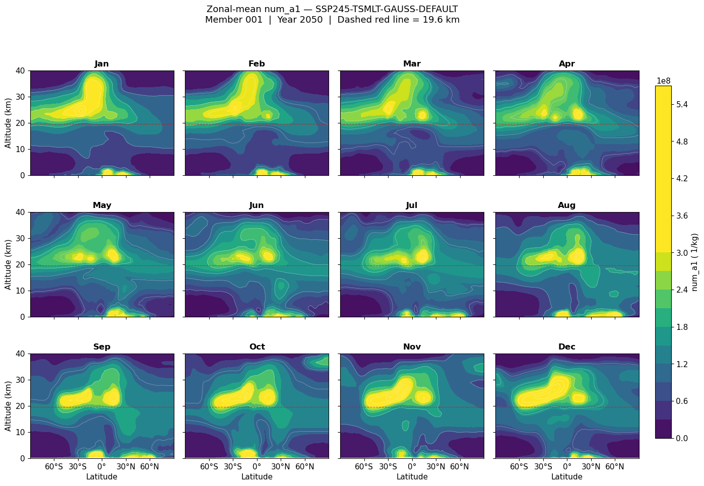
Saved plot : ./num_a1_zonal_mean_2050_001.png
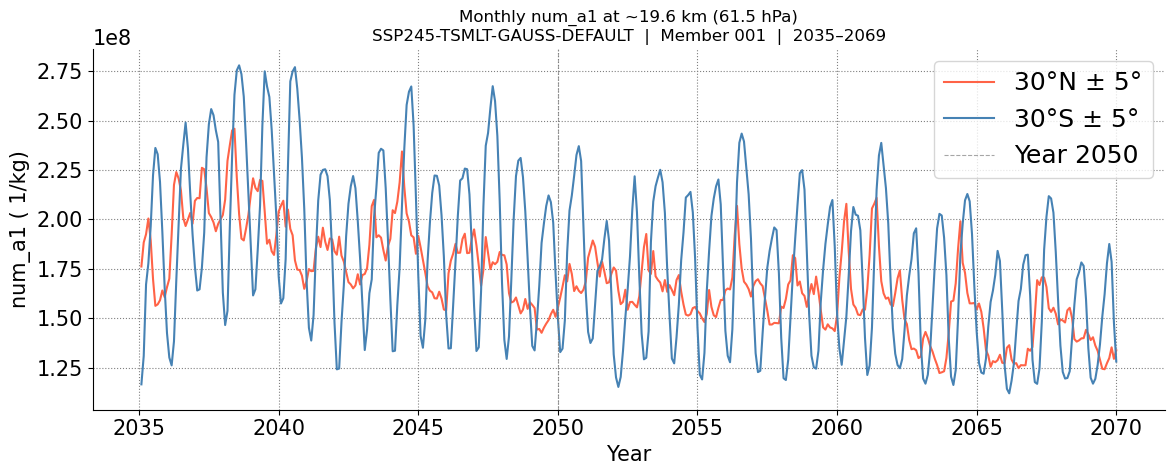
  Saved plot : ./num_a1_timeseries_20km_30N_30S_001.png
  Saved NC   : ./num_a1_timeseries_20km_30N_30S_001.nc
    → to load: xr.open_dataset("./num_a1_timeseries_20km_30N_30S_001.nc")
    → select year 2050: ds.sel(time=slice(2050.0, 2050.99))
    → select June 2050: ds.sel(time=2050+5/12, method="nearest")
    → by label:         ds.where(ds.time_label=="2050-06", drop=True)
  Memory freed.

============================================================
  Processing: num_a2
============================================================
  Opening: s3://ncar-cesm2-arise/ARISE-SAI-1.5/b.e21.BW.f09_g17.SSP245-TSMLT-GAUSS-DEFAULT.001/atm/proc/tseries/month_1/b.e21.BW.f09_g17.SSP245-TSMLT-GAUSS-DEFAULT.001.cam.h0.num_a2.203501-206912.nc
  Closest level to 20.0 km: 61.52 hPa  (19.61 km)
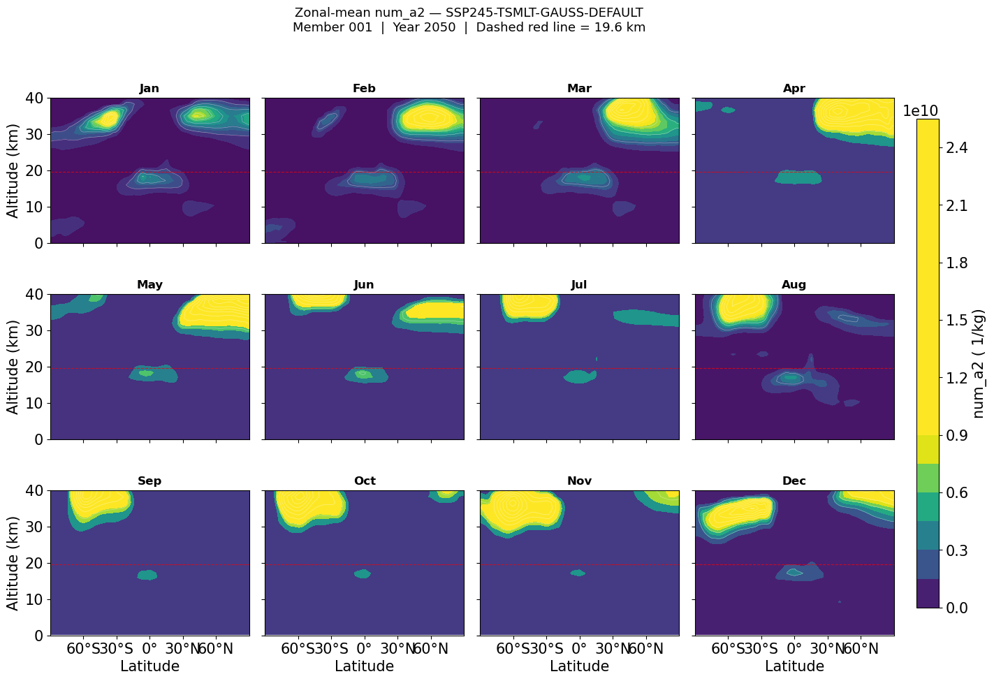
Saved plot : ./num_a2_zonal_mean_2050_001.png
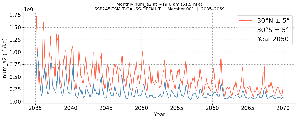
  Saved plot : ./num_a2_timeseries_20km_30N_30S_001.png
  Saved NC   : ./num_a2_timeseries_20km_30N_30S_001.nc
    → to load: xr.open_dataset("./num_a2_timeseries_20km_30N_30S_001.nc")
    → select year 2050: ds.sel(time=slice(2050.0, 2050.99))
    → select June 2050: ds.sel(time=2050+5/12, method="nearest")
    → by label:         ds.where(ds.time_label=="2050-06", drop=True)
  Memory freed.

============================================================
  Processing: num_a3
============================================================
  Opening: s3://ncar-cesm2-arise/ARISE-SAI-1.5/b.e21.BW.f09_g17.SSP245-TSMLT-GAUSS-DEFAULT.001/atm/proc/tseries/month_1/b.e21.BW.f09_g17.SSP245-TSMLT-GAUSS-DEFAULT.001.cam.h0.num_a3.203501-206912.nc
  Closest level to 20.0 km: 61.52 hPa  (19.61 km)
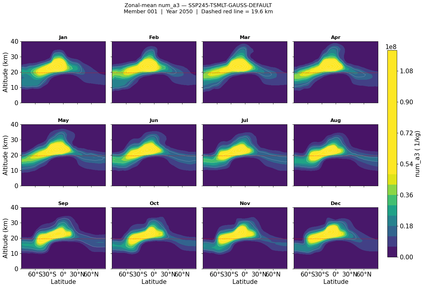
Saved plot : ./num_a3_zonal_mean_2050_001.png
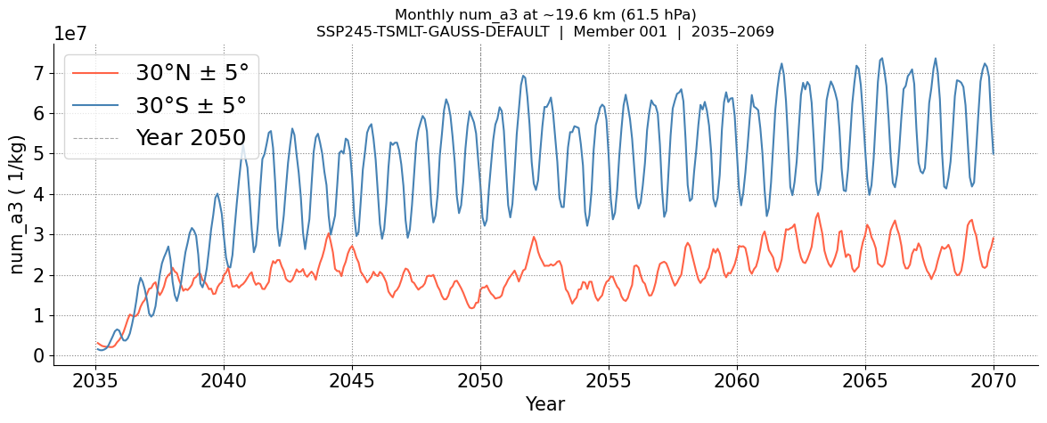
  Saved plot : ./num_a3_timeseries_20km_30N_30S_001.png
  Saved NC   : ./num_a3_timeseries_20km_30N_30S_001.nc
    → to load: xr.open_dataset("./num_a3_timeseries_20km_30N_30S_001.nc")
    → select year 2050: ds.sel(time=slice(2050.0, 2050.99))
    → select June 2050: ds.sel(time=2050+5/12, method="nearest")
    → by label:         ds.where(ds.time_label=="2050-06", drop=True)
  Memory freed.

============================================================
  All variables processed.
============================================================